When a controller needs tuning, what can a language model contribute?
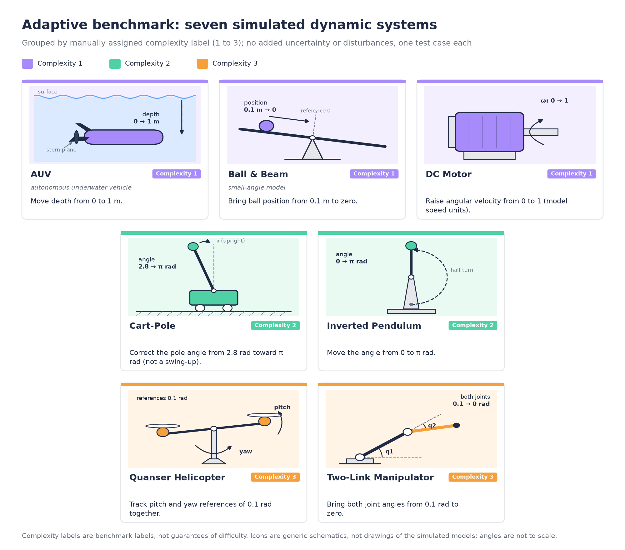
Inside LabCD's Adaptive control benchmark: understandable tasks, repeated trials, and a quality score that rewards good control without pretending every result is simply pass or fail.
Keeping a robot joint on target sounds simple until accuracy, speed, and actuator use start competing. A controller can move quickly but overshoot. It can move gently but take too long. A tuning change that helps one system may hurt another.
LabCD's Adaptive benchmark explores whether language models can help make those engineering choices. The language model helps select a supported control method and tune its parameters. A mathematical controller, not a chat response issued at every time step, then acts on the simulated system.
The saved results show generally high quality scores on this suite, but they also contain an important lesson: a polished average does not prove robustness, and a failed internal stopping check does not necessarily mean the physical response is poor.
What “Adaptive” means here
A plant is the system being controlled. Its states describe its condition, its inputs are actuator commands, and a controlled output is the quantity we want to bring to a reference. For a two-joint arm, for example, both joint angles can be controlled outputs even though the model also contains joint velocities.
The module supports structured nonlinear-control designs, including sliding-mode control and backstepping, when the model satisfies their requirements. Broadly, sliding-mode control builds a combination of tracking errors that should be driven toward zero; backstepping constructs a controller step by step for suitable chains of state equations. Some supported designs include adaptive terms intended to handle unmodeled effects.
These are not arbitrary control programs invented from scratch by each language model. The core provides the mathematical design and simulation machinery. A design agent selects a supported route, and a tuner proposes numerical parameters such as gains and adaptation settings. Candidate responses are evaluated, and the selected parameter set is verified again.
Inside LabCD's agentic Adaptive workflow
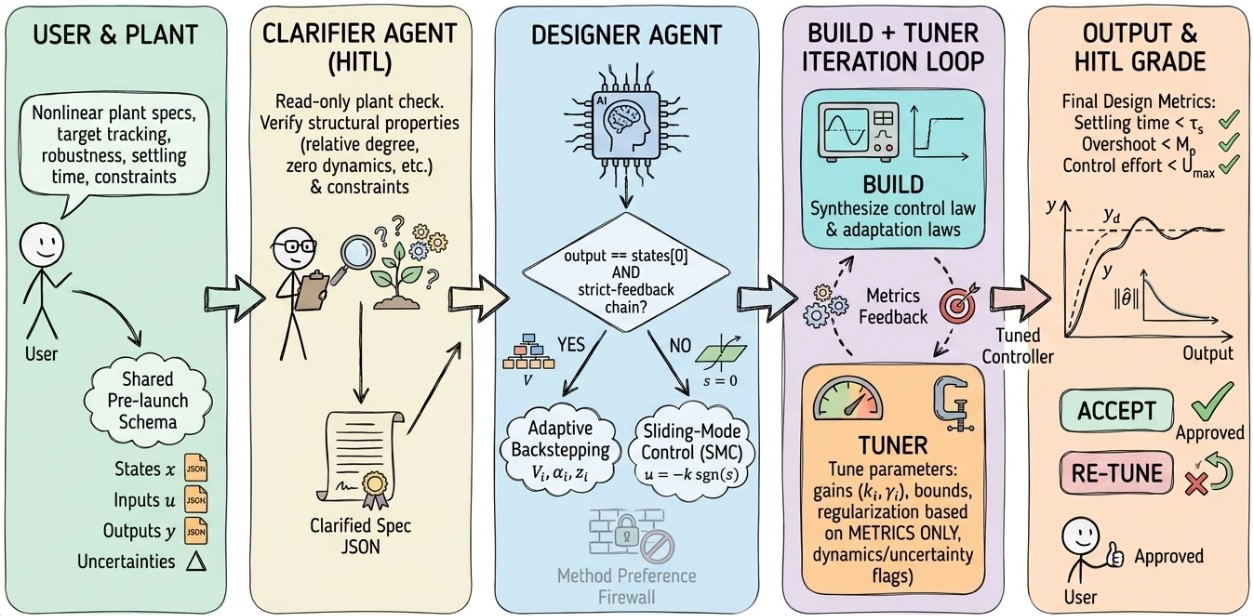
How the agent roles fit together. The user describes the plant and goals in a shared pre-launch schema of states, inputs, outputs and uncertainties. A clarifier agent runs a read-only plant check of structural properties and constraints, with a human in the loop, and produces a clarified spec. A designer agent checks whether the plant has a strict-feedback chain: if yes it routes to adaptive backstepping, if not to sliding-mode control, behind a method preference firewall. A build step synthesizes the control and adaptation laws, and a tuner adjusts gains, bounds and regularization based on metrics only. The tuned controller is reported against final design metrics, and the user accepts it or asks for a re-tune.
That distinction matters: identical-looking control-law structures can come from different LLM runs because they share the same underlying design family. The comparison is about the resulting tuned behavior, not whether each model invents a visually different equation. If the initial controller remains the best, that alone does not prove that no tuning was attempted.
Seven test systems and 105 saved runs
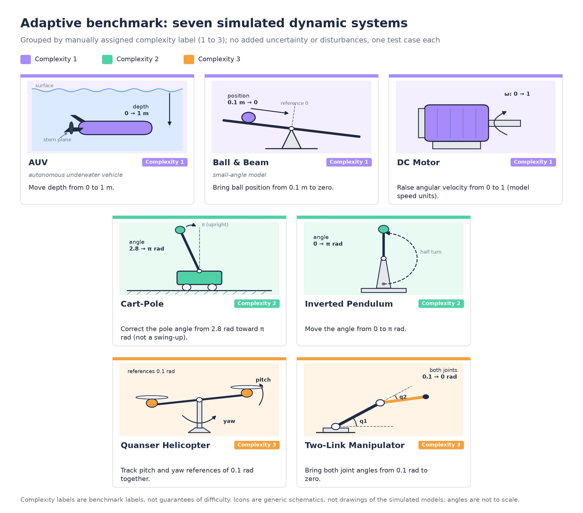
The seven simulated systems, colour-coded by their manually assigned complexity label. Icons are generic schematics, not drawings of the simulated models; angles are not to scale.
The suite contains one test per system and five language-model labels: GPT-5.4 Mini, GPT-5.4 Nano, GPT-4o Mini, GPT-4.1 Nano, and Groq GPT-OSS 120B. Each combination is repeated with seeds 42, 123, and 2024: 7 systems × 5 models × 3 seeds = 105 saved results. Mock-agent results are excluded.
A seed initializes supported random choices. Repetition helps reveal whether an observed result is consistent, but a seed is not a guarantee of identical behavior from an external model service.
| Complexity label | Simulated system | The controlled-output task |
|---|---|---|
| 1 | AUV, an autonomous underwater vehicle | Move depth from 0 to 1 metre. |
| 1 | Ball & Beam, small-angle model | Bring ball position from 0.1 metre to zero. |
| 1 | DC Motor | Raise angular velocity from 0 to 1 in the model's speed units. |
| 2 | Cart-Pole | Correct the pole angle from 2.8 radians toward π radians. This is not a swing-up starting from rest at the downward position. |
| 2 | Inverted Pendulum | Move the angle from 0 to π radians. |
| 3 | Quanser Helicopter | Track pitch and yaw references of 0.1 radians together. |
| 3 | Two-Link Manipulator | Bring both joint angles from 0.1 radians to zero. |
Complexity is a manually assigned grouping, not an objective score that guarantees which task will be hardest. The model equations, starting point, target, and scoring limits all affect difficulty.
The tests contain no added uncertainty or disturbances. In particular, the word “Adaptive” should not be read as evidence that this experiment establishes performance under unknown loads, noisy sensors, or parameter changes. Those require separate tests.
A softer way to judge the result: Success Rate 6
Success Rate 6 is a continuous quality score, not the fraction of runs that passed. An 88% score means a high average credit under the benchmark's chosen rules, not an 88% probability that a real robot will work safely.
It combines four categories:
| Category | What it asks |
|---|---|
| Tracking MSE | Across the full verification simulation, how large is each controlled output's average squared tracking error? |
| Overshoot | How far does an output cross beyond its reference, relative to its initial distance from that reference? Starting far away is not itself overshoot. |
| Settling time | How long does the simulator report that the response takes to enter and remain in its settling band? |
| Control effort | How large are the applied input commands, using their mean squared magnitude? This is not the LLM's dollar cost or necessarily physical energy. |
The benchmark assigns a reference limit, (L), to each measurement. These limits express the experiment's preferences, not universal engineering standards. For a nonnegative measurement (x) and positive limit:

You do not need the equation to read the results:
| Measurement compared with its limit | Credit for that measurement |
|---|---|
| At or below 60% of the limit | 100% |
| Exactly at the limit | About 82.03% |
| Twice the limit | 50% |
For a four-second settling limit, a genuinely settled response at or before 2.4 seconds gets full settling credit. At four seconds it gets about 82%; at eight seconds it gets 50%. A response that never settles gets zero settling credit, even if the simulator reports the simulation duration as a fallback number.
MSE and overshoot are scored separately for each declared controlled output, then averaged within their category. The four enabled category credits receive equal weight. This avoids giving the two-output systems twice the category weight of the one-output systems. Numerical failures force zero credit; unavailable required measurements remain unavailable. All 105 selected records have an available score.
Which tasks distinguish the language models?
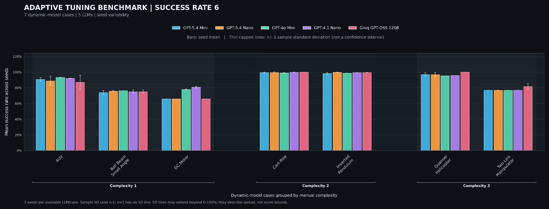
A bar is the mean of three seeds for one language model and system. A thin capped line shows one sample standard deviation: how much those repeats vary. It is not a confidence interval or a guarantee about future runs.
The results do not follow a simple “higher complexity means lower quality” rule:
- Cart-Pole and Inverted Pendulum score close to 100% across the compared models. For Cart-Pole, remember that the pole starts at 2.8 radians, already relatively close to its π-radian reference. This is a different task from lifting it from the downward resting position.
- DC Motor separates the models more clearly. GPT-4.1 Nano averages about 80.86%, GPT-4o Mini about 77.99%, and the other three labels about 65.82% on this case.
- The two-joint manipulator is not a solved-by-everyone story. Four model means fall between 77.01% and 77.04%, while Groq averages about 81.56%. That is a task-specific observation, not evidence that one model is universally superior.
Short error lines indicate consistent scores across these repeats; they do not establish that the controller is correct under untested conditions. Three seeds are useful for a first view of variability, but too few to turn small differences into strong statistical claims.
Quality and LLM cost are different questions
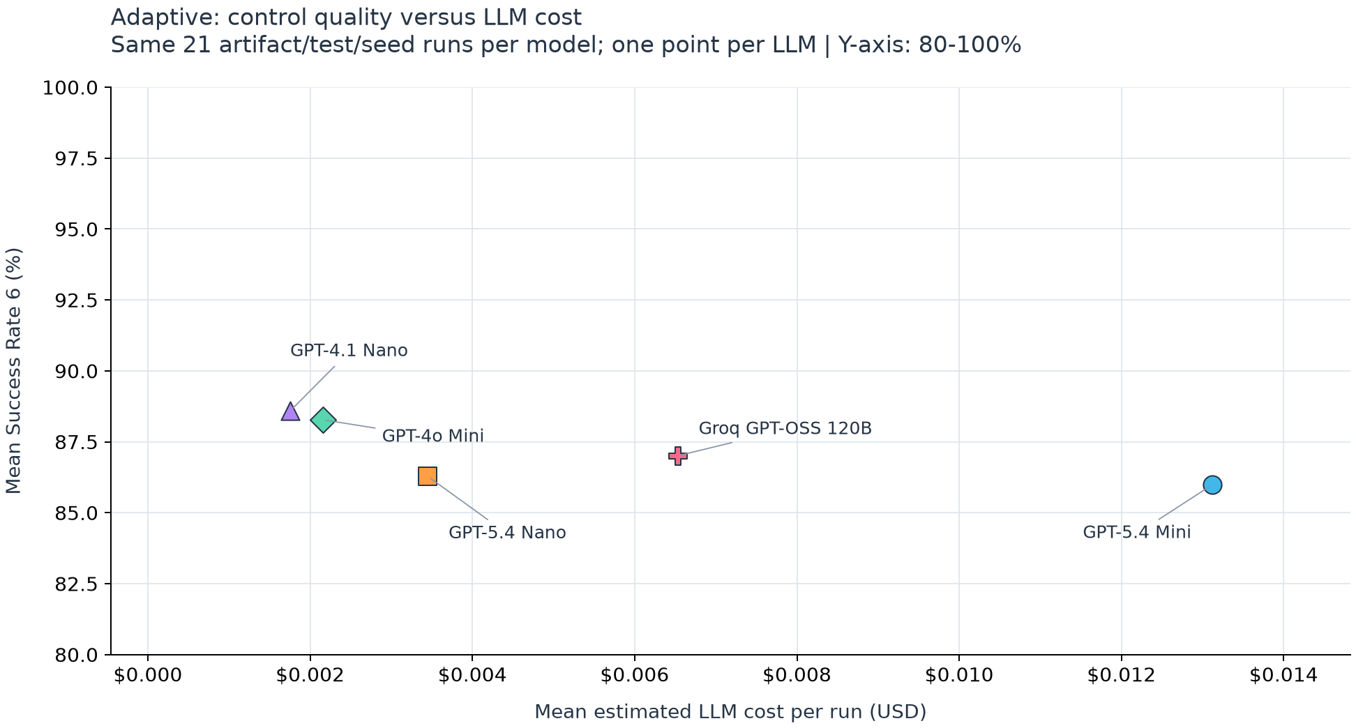
Each point represents one language model over the same 21 case/seed combinations. Higher means better average quality; further left means lower estimated LLM cost. The vertical axis intentionally starts at 80%, not zero; read the numerical differences as well as the positions.
| Saved model label | Mean Success Rate 6 | Mean estimated LLM cost per run |
|---|---|---|
| GPT-5.4 Mini | 85.99% | $0.013121 |
| GPT-5.4 Nano | 86.29% | $0.003448 |
| GPT-4o Mini | 88.28% | $0.002155 |
| GPT-4.1 Nano | 88.59% | $0.001755 |
| Groq GPT-OSS 120B | 87.01% | $0.006531 |
GPT-4.1 Nano has the highest suite-average score and the lowest estimated mean cost in this saved set. But its quality lead over GPT-4o Mini is only about 0.31 percentage points. That is a narrow observed difference, not a demonstrated statistically significant advantage.
The cost figures are historical estimates from saved token usage and local pricing, not current quotes or invoices. They can reflect different numbers and lengths of agent calls, and they exclude simulation compute and engineering effort. Nothing here establishes that a more expensive LLM necessarily produces a better controller.
Reading a real saved response
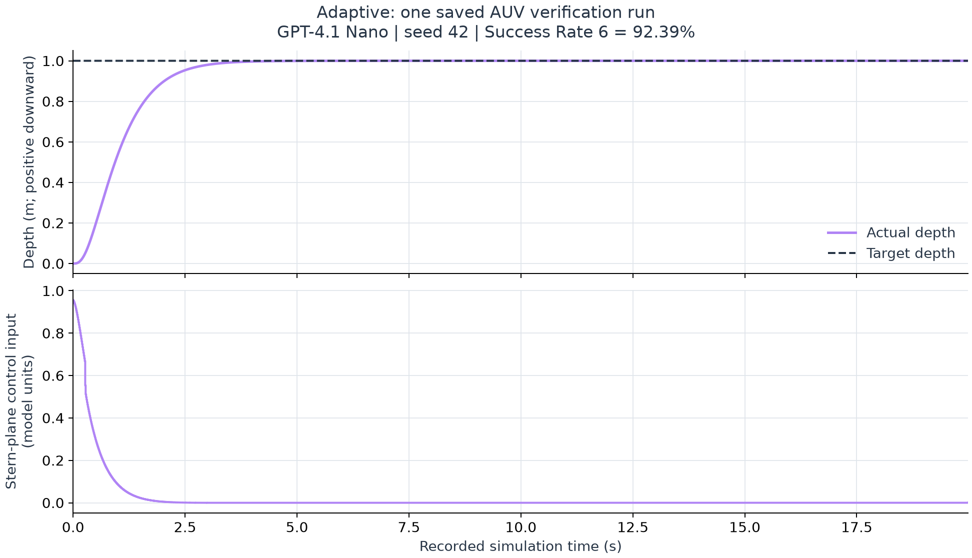
Illustrative run: GPT-4.1 Nano, seed 42, AUV. This is one explicitly identified run, not an average, not a newly executed simulation, and not a claim that all systems behave this way.
The purple depth trace approaches the dashed one-metre reference. The lower panel shows the command that achieves that movement. Looking at both prevents a misleading interpretation: reaching the reference is not enough if doing so requires excessive or rapidly changing commands.
The run's Success Rate 6 is 92.39%. Its category credits are approximately 93.99% tracking, 92.84% settling, 100% overshoot, and 82.73% effort. Their average gives the headline score. It earns less than full credit even though its measurements meet their reference limits, because full credit applies only in the more demanding 60%-of-limit allowance region.
Why can a good response still have a native “fail” verdict?
The saved Adaptive experiment uses a particularly strict tuning-stop target: target_steady_rms_fraction = 0.0. This asks for exactly zero computed normalized RMS error in the final part of the simulation. RMS is the square root of average squared error; normalization expresses it relative to the task's scale.
Tiny positive numerical errors can therefore fail the core's stopping check even when the response is extremely close to the reference. The AUV example above has a native verification.success = false while still receiving 92.39% under Success Rate 6.
That is not a contradiction. The native verdict answers a strict stopping question; the offline score answers a broader quality question using full-window tracking, overshoot, settling, and input use. Neither should be silently substituted for the other, and zero tolerance is a diagnostic choice, not a realistic universal accuracy requirement.
What these results do and do not establish
The practical message is that language models can be compared as assistants within a structured controller-design and tuning workflow. Their suggestions can lead to different control behavior and different token spending, even when the mathematical form of the controller is shared.
There are important limits to this evidence. The tests are simulated and nominal. Native settling rules differ from MPC's, and the Adaptive path does not enforce MPC's actuator bounds. Ball & Beam uses a small-angle approximation and a 0.1-metre initial displacement, whereas the MPC artifact uses the nonlinear input model and a 1-metre displacement. Aircraft Pitch and CSTR are absent from this active Adaptive suite. Consequently, the suite-average Adaptive score is not an apples-to-apples victory over the MPC suite.
More informative next tests would keep task definitions matched where feasible, add realistic uncertainty and actuator constraints, use more seeds, and inspect both the trajectory and the input whenever a headline score looks unusually good.
Try it on your own system. Bring a model or IO data for a bounded control problem and run LabCD's guided workflow on your first model for free at app.labcd.ai. A qualified engineer keeps approval of every controller.
Data and portability note. Prepared on 23 October 2026 from the saved Adaptive batch 2026-10-17_17h. The folder's timestamp records archive organization, not a verified original experiment date. The case chart is copied from the saved Rate 6 figure and checked against its CSV and JSON results. The cost and AUV figures use saved data only; no tuning, simulation, or API calls were rerun. Figure provenance and numerical summaries accompany this post. Keep assets/adaptive beside this Markdown file when publishing or moving it; reading the post does not require a running LabCD installation or the other article.
Want to try this on your own plant model?
Try LabCD free with your first model