Can a language model help tune a controller that looks ahead?

A practical look at LabCD's model predictive control benchmark, with simulated systems, repeated runs, and an honest account of what the results mean.

Imagine steering a vehicle toward a bend. A useful driver does not wait until the car has left the road to react: they look ahead, anticipate what will happen, and adjust the steering and speed. Model predictive control, or MPC, follows a similar idea using a mathematical model.

But an MPC controller still needs good settings. How far should it look ahead? How strongly should it prioritize accuracy over using less actuator input? This benchmark asks whether language models can help choose those settings, and whether the resulting controllers actually behave well in simulation.

The short answer from this saved experiment is that the language model matters, but so does the task. A model that does well on one system is not automatically the best on another. A single average is useful, but not sufficient.

First, what is being controlled?

A plant is simply the system we want to control: a motor, a robot arm, or a simulated vehicle. Its states describe its current condition, such as position and velocity. An input is the command applied to it, such as voltage, torque, or a steering-surface command. A reference is the desired value of a selected output.

MPC repeatedly predicts possible future behavior, chooses an input sequence, applies its first command, and plans again using the updated state. Declared bounds can limit the allowed commands or states. The prediction horizon determines how far ahead it considers; numerical weights determine the trade-off between competing objectives.

The language model is not queried for every actuator command. It proposes controller settings between simulation evaluations. The numerical MPC controller then computes the commands during each simulation. This separates the language model's engineering suggestions from the controller's real-time calculations.

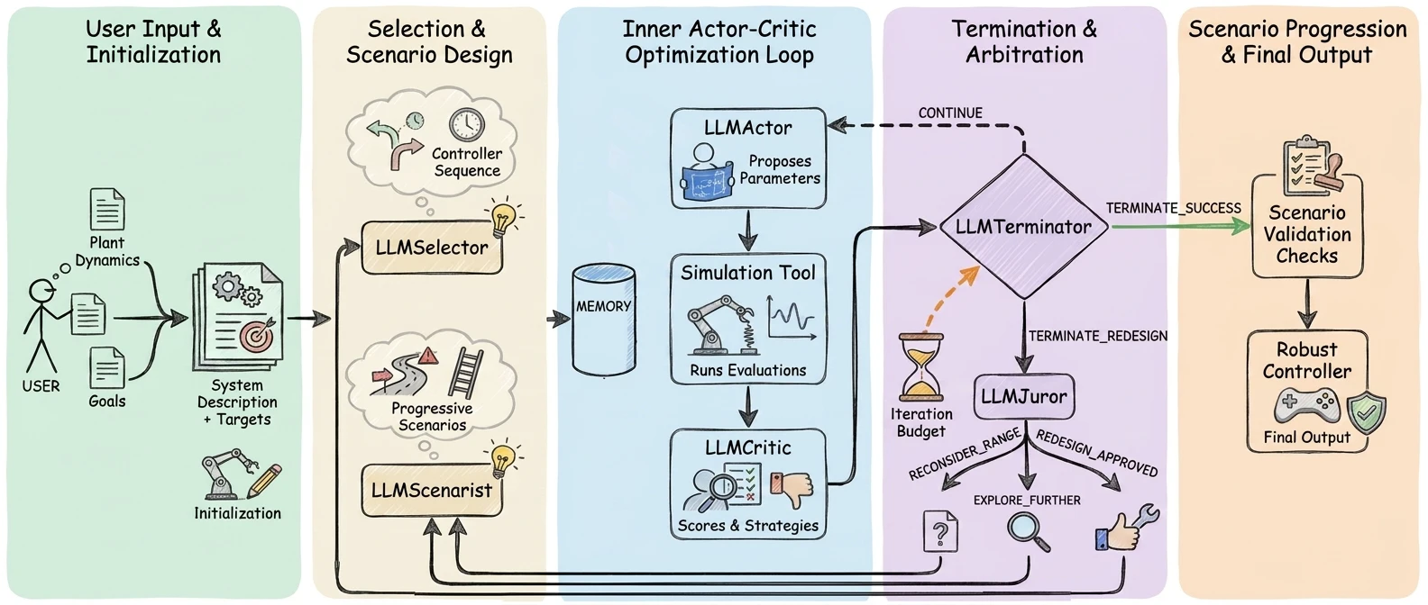
In LabCD, agent roles propose settings, evaluate the simulated response, critique it, and review whether tuning should continue. A separate verification simulation checks the selected controller. The saved reports contain evaluated tuning runs with up to 20 recorded iterations; not every run uses the same number.

Inside LabCD's agentic MPC workflow

How the agent roles fit together. The user supplies plant dynamics and goals. A selector chooses the controller sequence and a scenarist designs progressive scenarios. In the inner loop, an actor proposes parameters, the simulation tool runs evaluations, and a critic scores the result and suggests strategies, with shared memory across iterations. A terminator decides whether to continue, stop with success, or ask for a redesign within the iteration budget; a juror reviews redesign requests. Scenario validation checks run before the final controller is output.

The experiment: nine systems, five language models, three repeats

Each system has one test case. Every language model runs every case with seeds 42, 123, and 2024, giving 135 saved results: 9 cases × 5 models × 3 seeds. A seed initializes supported random choices; it does not guarantee identical replies from a remote language-model service.

The five saved model labels are GPT-5.4 Mini, GPT-5.4 Nano, GPT-4o Mini, GPT-4.1 Nano, and Groq GPT-OSS 120B. Mock-agent results are not included.

Complexity label	Simulated system	The controlled-output task
1	AUV, an autonomous underwater vehicle	Move depth from 0 to 1 metre.
1	Ball & Beam	Move a ball from 1 metre to the reference position at zero.
1	DC Motor	Raise angular velocity from 0 to 1 in the model's speed units.
2	Cart-Pole	Move the pole angle from 2.8 radians toward π radians, not a swing-up from a downward resting position.
2	Inverted Pendulum	Move the angle from 0 to π radians.
3	Quanser Helicopter	Track pitch and yaw references of 0.1 radians together.
3	Two-Link Manipulator	Bring both joint angles from 0.1 radians to zero.
4	Aircraft Pitch	Track a pitch-angle reference of 0.0948 radians in the longitudinal aircraft model.
4	CSTR, a continuously stirred tank reactor	Move reactor temperature from 4.5 to 5 in the model's temperature scale; these numbers are not a Celsius claim.

These complexity levels are manually assigned benchmark labels, not physical laws or guarantees of difficulty. More states and inputs can make a task harder, but initial conditions, targets, actuator authority, and scoring limits also matter. The aircraft and reactor models also have non-zero trim inputs: baseline commands needed to maintain their operating points.

The artifact definitions request a nominal scenario: no added measurement noise or physical-parameter perturbation. This is a controlled starting point, not a test of every real-world disturbance.

What does “Success Rate 6” actually measure?

Despite its name, Success Rate 6 is a continuous control-quality score, not the percentage of tests that passed. A score of 90% does not mean “90% of runs succeeded,” nor does it prove safety or stability.

It combines four questions:

Category	Plain-language meaning
Tracking MSE	Over the full verification simulation, how large is the average squared error in each declared controlled output? Smaller is better.
Overshoot	How far does each controlled output cross beyond its reference, relative to its initial distance from that reference? Smaller is better.
Settling time	How long does the simulator report that the response takes to satisfy its settling check? A run that never settles receives no credit for this category.
Control effort	How large are the applied commands on average, measured using squared inputs? This is not the LLM's dollar cost and is not automatically physical energy.

Each measurement is compared with a case-specific reference limit, (L). Those limits are benchmark choices, not universal engineering acceptance standards. For a nonnegative measurement (x) and a positive limit, the saved score uses:

$$ s(x,L)=2^{-\max\left(0,\frac{x/L-0.60}{2.00-0.60}\right)}. $$

In everyday terms:

Measurement compared with its limit	Credit for that measurement
At or below 60% of the limit	100%
Exactly at the limit	About 82.03%
Twice the limit	50%

For example, with a 5% overshoot limit, overshoot up to 3% earns full credit. At 5% it earns about 82%, rather than suddenly falling from full credit to zero.

For systems with two controlled outputs, their MSE credits are averaged within the tracking category; overshoot is handled similarly. The four enabled category credits then receive equal weight. Each saved run therefore has one score. Numerical failures force zero credit; missing required evidence leaves a score unavailable rather than silently turning it into zero. All 135 selected records have an available score.

The scope matters: tracking MSE and overshoot use only the declared controlled outputs, while settling uses MPC's existing check on the combined error across all states. It is not a separate settling calculation for each selected output.

What the system-by-system results show

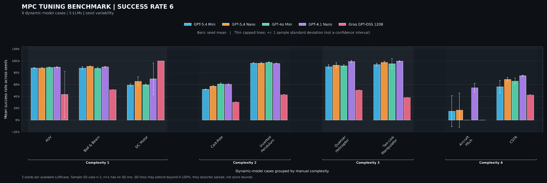
Each color identifies a language model. A bar is the mean of three seeds for that model and case. Thin capped lines show one sample standard deviation, a measure of repeat-to-repeat spread, not a confidence interval.

Three observations stand out:

• The strongest overall average does not imply winning every case. GPT-4.1 Nano has the highest mean across this nine-case suite, but GPT-5.4 Nano scores about 90.98% on Ball & Beam, and Groq GPT-OSS 120B records 100% on DC Motor.
• Complexity is not a staircase of inevitable failure. Several models score strongly on the helicopter and manipulator even though those systems have multiple interacting channels. Cart-Pole is less successful despite its lower label.
• Aircraft Pitch is a warning against relying only on an average. Its case means range from about 0.05% to 54.62% across these models. That is a substantial unresolved weakness in this particular experiment, not evidence of deployment-ready aircraft control.

Some MPC error lines extend below 0% or above 100%. The individual scores do not: the lines display “mean ± standard deviation,” which is not a bounded range of possible scores. With only three seeds, the spread is descriptive evidence, not a precise statistical ranking.

Does more LLM spending buy better control?

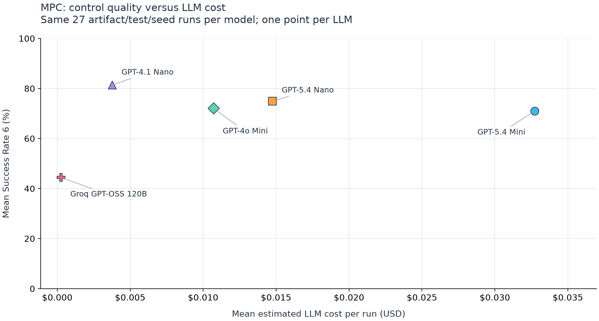
Moving upward means higher mean control quality; moving left means lower estimated LLM spending. Each point averages exactly the same 27 case/seed combinations for one model.

Saved model label	Mean Success Rate 6	Mean estimated LLM cost per run
GPT-5.4 Mini	70.99%	$0.032724
GPT-5.4 Nano	74.90%	$0.014756
GPT-4o Mini	72.06%	$0.010709
GPT-4.1 Nano	81.43%	$0.003772
Groq GPT-OSS 120B	44.41%	$0.000262

There is no simple “spend more, get better control” pattern here. GPT-4.1 Nano has both the highest suite-average score and a lower estimated mean cost than several alternatives. Groq has the lowest estimated cost, but its high DC Motor score does not carry across the whole suite.

These are saved token-cost estimates, not current price quotations or verified invoices. Runs may make different numbers of calls, so cost reflects the workflow as well as the model. It excludes simulation compute, electricity, and engineering time. Different model versions, pricing tables, or tuning budgets could change the picture.

What a good-looking response looks like

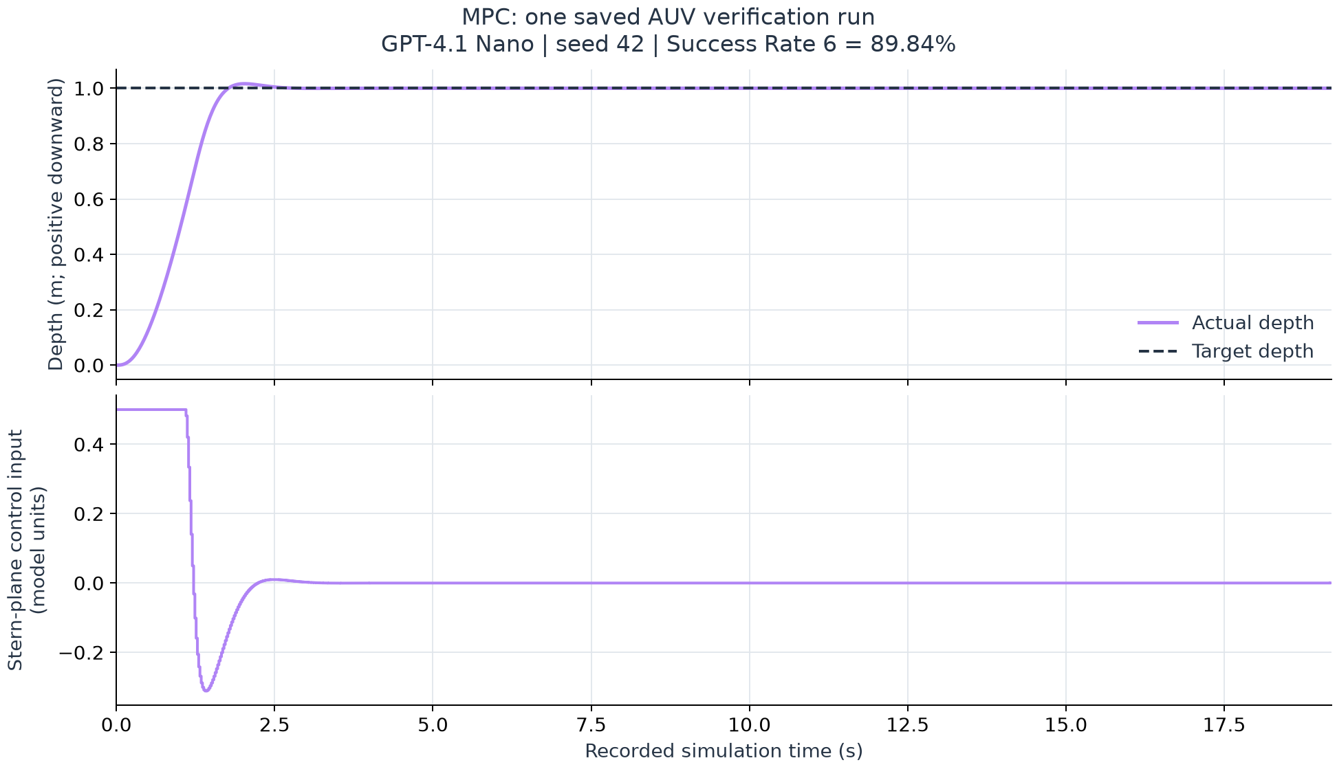
Illustrative run: GPT-4.1 Nano, seed 42, AUV. This is one named run, not a seed average, not the best run selected from the suite, and not a newly executed simulation.

The dashed line is the desired depth; the purple line is actual depth. The lower panel shows the command that produces the motion. The vehicle approaches one metre, crosses the target slightly, then stays close while the input returns near zero.

Its score is 89.84%, rather than 100%, because the final number evaluates the whole response and its input use. In this run the four category credits are approximately 90.05% tracking, 100% settling, 100% overshoot, and 69.31% effort. Their average explains the headline score. A response that looks accurate can still demand more control input than the benchmark prefers.

The useful takeaway, and the boundary of the claim

This benchmark is encouraging as a test of LLM-assisted tuning, not a demonstration that a language model can replace control engineering. It shows why both task-level results and repeatability matter, and why control quality and token spending should be reported together.

The boundaries are important: these are simulations, each case has only three seeds, complexity labels and limits are manually chosen, and the artifacts describe nominal conditions. Completing a tuning workflow is not the same as meeting every control objective. Nor should this suite's average be compared directly with another controller's average when the case lists, initial conditions, models, or constraints differ.

The next useful evidence would be more repeats, matched task definitions, explicit disturbance tests, and examination of the lowest-scoring cases, not simply a larger headline average.

Try it on your own system. Bring a model or IO data for a bounded control problem and run LabCD's guided workflow on your first model for free at app.labcd.ai. A qualified engineer keeps approval of every controller.

---

Data and portability note. Prepared on 23 October 2026 from the saved MPC batch 2026-10-18_12h. That folder records archive organization time, not a verified original experiment date. The system-by-system chart is copied from the saved Rate 6 figure and checked against its CSV and JSON results. The cost and AUV figures are rendered from saved results only; no tuning, simulation, or API calls were rerun. Figure provenance and numerical summaries accompany this post. Keep the assets/mpc folder beside this Markdown file when publishing or moving it; no running LabCD installation is needed to read it.